Encoding the $2d$ Ising Model onto $1d$ Qubit Chains
Table of Contents
The $2d$ Ising model is perhaps the most well recognized model in condensed matter and statistical physics and described by the Hamiltonian $$ H = -\sum_{\langle i,j\rangle}\tilde{J}_{ij}S_i S_j $$
where classical spins $S _k \in \{-1, 1\}$ rest on each lattice site $i\in\Lambda _{2}$ and interact with their nearest neighbors $\langle i,j\rangle$ with strength $\tilde{J} _{ij}$.
Recently, I was studying phase transitions in the TFIC and, as it turns out, the above Hamiltonian for the $2d$ classical Ising model is dual to the quantum transverse field Ising chain (TFIC) formed out of qubits with the Hamiltonian $$ \hat{H} = - {J}\bigg[\sum _{\langle i,j \rangle}{Z}_i{Z}_j + g \sum_k {X}_k \bigg] $$ where $g$ denotes the magnetic moment of the transverse magnetic field, $J$ sets the overall energy scale, and ${X},{Z}$ are the Pauli spin matrices in the denoted directions.
Dualities are a type of correspondence where one can map two (seemingly different systems) onto each other. As dualities translate hard problems from one system into more tractable problems in the other, one can draw rich physical insights from utilizing them and the $2d$ Ising model is no exception.
Here, I first show how one can map the $1d$ classical Ising chain onto a single qubit in an external magnetic field before constructing qubit chains from the $2d$ Ising model. Along the way, we will write a formal statement of what justifies a duality, establish the the dictionary between the two systems $(\tilde{J} _{ij} \leftrightarrow ({J},g))$, and identify the physical insights one can draw when utilizing dualities.
Encoding the $1d$ Classical Ising Model onto a Qubit #
The $1d$ classical Ising model is either a line or chain of classical spins depending if one has free or periodic boundary conditions. Here, I assume periodic boundary conditions on a chain of $N$ spins, denoted by $\bigcirc$, which can be modeled by the Hamiltonian $$ H^{\bigcirc} \equiv H _{{\rm Ising} _{1d}} = - \tilde{J} \sum _{i=1}^N S _i S _{i+1} $$ where the interaction strength has been assumed to be uniform. The $2^N$ configurations can be represented by the partition function $$ \mathcal{Z}^\bigcirc \equiv \mathcal{Z} _{\textrm{Ising} _{1d}} = \sum _{\{ S \}}e^{-\beta _\textrm{Ising} H(S)} = \sum _{\{S\}}\exp\left(K\sum _{i=1}^N S _i S _{i+1}\right) $$
where $K = \beta_{\rm Ising} \tilde{J}$.
The Transfer Matrix #
Now, we employ the transfer matrix method. The trick is to write $\mathcal{Z}^\bigcirc$ as a trace over a matrix product. To facilitate this, let’s first complete the square
$$ \mathcal{Z}^\bigcirc = e^{K N}\sum _{\{S\}}\exp\left(-\frac{K}{2}\sum _{i=1}^N [S _i - S _{i+1}]^2 \right) = e^{KN}\sum _{\{S\}}\prod _{i=1}^N e^{-\mathcal{L}(i,i+1)} $$
where I have used that the residual term $\sum_{i}(S _i^2 + S _{i+1}^2) = 2N$ since each spin belongs to $S_i \in \{-1,1\}$.
This is the intuition behind the transfer matrix1. The matrix elements are determined by the value of the spin at the lattice site. For $S _i=S _{i+1}$, one obtains $T(i,i+1) = 1$ where as when $S _i=-S _{i+1}$, one obtains $T(i,i+1) = e^{-2K}$. The upshot is then that $$ T(i,i+1) = \begin{pmatrix}1 & e^{-2K} \newline e^{-2K} & 1\end{pmatrix} _{i,i+1}= \langle S _i| \mathbf{T}|S _{i+1}\rangle $$ where in the last equality, we interpret $\mathbf{T}$ as an operator acting on a two level quantum system! Hence, one obtains
$$ \begin{align*} \mathcal{Z}^\bigcirc &= e^{KN}\sum _{\{S\}}\prod _{i=1}^N e^{-\mathcal{L}(i,i+1)} = e^{KN}\sum _{\{S\}}\prod _{i=1}^N T(i,i+1)\newline & = e^{KN}\sum _{S _1 = \pm1}\cdots \sum _{S _N = \pm1}\langle S _{1}|\mathbf{T}|S _{2}\rangle\cdots \langle S _{N}|\mathbf{T}|S _{N+1}\rangle \newline & = \sum _{S _1 = \pm 1} \langle S _{1}|(e^{K}\mathbf{T})^N|S _{N+1}\rangle = \textrm{Tr}(\mathbf{t}^N). \end{align*} $$
The Qubit Hamiltonian #
The last step to encode the classical Ising chain is to demand that $\mathbf{t}^N$ is equal to the new Hamiltonian ${\hat{H}^\odot}$ for a single qubit, denoted by $\bigodot$, evolving in Euclidean time $\beta = N \delta \tau$ in a transverse field. First, we notice that the transfer matrix $\mathbf{t}$ satisfies $$ \mathbf{t} = e^{K}(\mathbb{I} + e^{-2K}X) $$ where $X$ is the Pauli matrix.
Since for an isolated qubit, the operators $(\mathbb{I},X,Y,Z)$ span the set of Hermitian operators, we can start with an ansatz that $$ -\delta\tau\hat{H}^\odot = a\mathbb{I} + bX $$ Recalling that $e^{a\mathbb{I}}= e^{a}\mathbb{I}$ and that $e^{bX} = (\cosh(b)\mathbb{I}+\sinh(b)X)$ we have $$ \begin{align*} e^K (\mathbb{I} + e^{-2K} X) = \begin{pmatrix}e^K & e^{-K} \newline e^{-K} & e^K\end{pmatrix} = e^a(\cosh(b)\mathbb{I}+\sinh(b)X) \end{align*} $$ which can be solved to set $e^{-2K} = \tanh(b)$ and $e^a = 2\sinh(K)\cosh(K)$. Hence we arrive at the Hamiltonian $$ \boxed{\hat{H}^\odot = -E_g \mathbb{I} - \frac{\Delta}{2}X} $$ where $E_g = {a}/{\delta\tau}$ is identified as the ground state energy and $\Delta = {2b}/{\delta \tau}$ is the energy gap which sets the magnetic moment of the transverse magnetic field via $\Delta = 2 J g.$
Physical Checks #
Let’s do a quick sanity check. We started with the 1D Ising model and claimed that we can map it onto a Hamiltonian for a single qubit. If so, then there should be no $Z_iZ_{i+1}$ interaction terms as there are no other qubits in the picture and all self interactions contribute to the ground state energy. We can identify the ground state energy using the Ising temperature $K = \beta _\textrm{Ising} \tilde{J}$. By sending, $K\to\infty$ $(\beta _\textrm{Ising} =({T _\textrm{Ising}})^{-1} \to \infty)$, one sends $b\to 0$ and $a\to\infty$ in which case we have $$ \hat{H}^\odot \approx -E_g\mathbb{I}. $$ Hence, at zero Ising temperature, we see that $E_g$ must be the correct ground state energy and there is no magnetic field. In the presence of a magnetic field, i.e., finite Ising temperature, there is an energy gap set by $\Delta$. The absence of any finite Ising temperature phase transition for the qubit is clearly related to the lack of a transition for the $1d$ Ising model.
As a bonus, it is straightforward to evaluate the partition function in this case by diagonalizing $\mathbf{t}$ and using the cylicity of the trace: $$ \textrm{Tr}(\mathbf{t}^N) = \lambda _+^N + \lambda _-^N = 2^N(\cosh(K)^N + \sinh(K^N)) $$
Encoding the $2d$ Classical Ising Model onto Qubit Chains #
The calculations for the $2d/1d$ are somewhat involved but can be found in several resources (see here2). The main idea can be more effectively communicated in the following graphic
Essentially, one takes the spins on each Euclidean timeline of the lattice and maps these states onto a single qubit. By repeating this process, the qubits form a chain with the interactions along the $x$ direction provided by the coupling strength $K_x$ as seen in the $2d$ Ising Hamiltonian $$ H _{2d\textrm{ Ising}}= \sum _{\langle i,j\rangle} K _x S _j(i)S _{j+1}(i)+ K _\tau S _j(i)S _j(i+1) $$ where $i,j$ spans the $\tau,x$ directions respectively. The duality (given by the blue line) essentially reads/encodes the spatial state of the lattice at a given time slice and prints it accordingly onto the qubits. The end result is that one has a unitary evolution with the $1d$ qubit chain Hamiltonian being $$ \hat{H} _{1d \textrm{ QC}} = - J \left(\sum _{i}Z _iZ _{i+1} + g\sum_i X_i\right). $$
From the resources quoted above, it turns out that the parameters are related via $$ K_x = J\delta \tau\hspace{.4in}e^{-2K_\tau} = \tanh(gK_x) $$
Phase Transitions and Entanglement #
You may (rightfully) object that I’ve clickbaited you by not providing the mathematics. Fret not! Instead, I’ll justify the above duality with some physics instead.
Magnetization #
For a square lattice, Onsager found the mean magnetization for the $2d$ Ising model to be $$ M = (1 - [\sinh(2K_\tau)\sinh(2K_x)]^{-2})^{1/8} $$ With the phase transition occurring at $\sinh(2K_\tau)\sinh(2K_x)=1$. Now, via the duality, we also have the mean magnetization $$ M_Q = \frac{1}{N}\langle\textrm{gs}|\hat{M}|\textrm{gs}\rangle $$ where $\hat{M}$ is the magnetization operator and $|\textrm{gs}\rangle$ refers to the ground state of the spin chain. Via the duality, we should expect that the phase transitions happen at the same location in the large $N$ limit and this can be easily checked (see my code here)
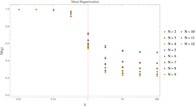
Clearly, there appears to be a phase transition around $g\approx 1$. For small coupling values, the spins are all anti-aligned with the external magnetic field hence $M_Q\approx 1$. At larger couplings, the spins flip to be aligned with the external field thereby becoming paramagnetic with $M_Q\to0$ in the large $N$ limit. The trend can be confirmed for larger qubit chains, but the computational time is prohibitive.
Entanglement Entropy #
A well known property of the $2d$ Ising model is that near the critical point $g=1$ it becomes a particular type of $2d$ conformal field theory. One of the most important tests for any duality is to be able to recover the entanglement structure on both sides. Thanks to Cardy and Cabreses, we know what the entanglement entropy for $2d$ conformal field theories is $$ S_{2d \textrm{ CFT}} = A + \frac{c}{3}\log\left(\frac{N}{\pi}\sin\left(\frac{\pi x}{N}\right)\right). $$ The parameters $A$ is an arbitrary shift which is dependent on the details of the entanglement surface and $c$ is a universal term, the central charge, which is known to be $c _\textrm{Ising}=1/2$ for the Ising model.
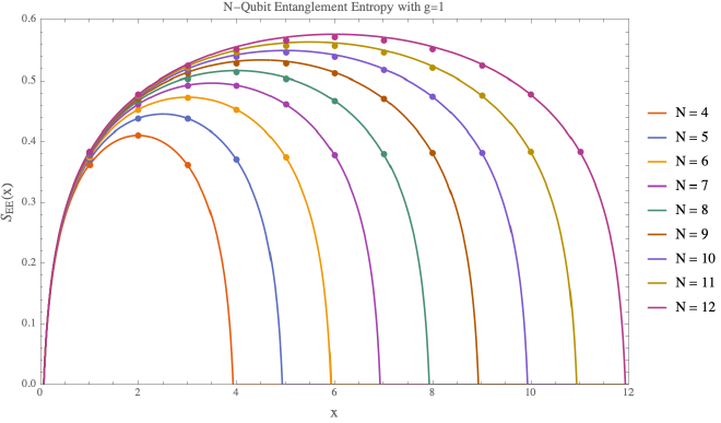
In the above, I plot the entanglement entropy for $2d$ CFTs and compare this against some code that I wrote (see here) which performs partial traces at locations $x$ on a qubit chain.
Clearly the CFT result matches precisely with the entanglement entropy calculated for $g=1$. In the large qubit limit, the central charge was numerically calculated to be $c \approx .518$ and should approach the CFT result with larger qubit chains.
Duality Protocols #
The $1d/0d$ classical/quantum Ising correspondence highlighted the formal equivalence between two systems and can be generalized into the following protocol
- Absorb the thermodynamic temperature $\beta _{{\rm Ising}}$ of the Ising model into the interaction strengths $\tilde{J} _{ij}$.
- Set the boundary conditions and interaction strengths to be equivalent along the lattice axes (this is another way of applying translation invariance along the lattice axes).
- Denote one of the $(d+1)$ spatial directions as Euclidean time, $\tau$, and consider the partition $N\delta \tau = \beta$ as the quantum temperature.
- Apply the transfer matrix to convert the partition function of a thermodynamic system into the path integral of a quantum system evolving in Euclidean time.
Obviously, the last step is the tricky leap in intution, but in the cases where this can be applied, we arrive at the formal equivalence between the partition functions of the two systems:
$$ \boxed{\mathcal{Z} _{(d+1)\textrm{ Ising}}(K _\tau,K _{x^d}) = \mathcal{Z} _{d \textrm{ TFIC}}(J _{x^d},g)} $$
where $K_\tau$ is the interaction strength along the Euclidean time direction and $K _{x^d}$ in the remaining spatial directions. The precise map between these parameters and those in the TFIC are given by the following dictionary.
The Dictionary between the Classical/Quantum Ising Models #
When mapping the $1d$ Ising model onto a qubit, we found that the coupling constant $K = \beta _\textrm{Ising} \tilde{J}$ was related to the parameters $(J,g)$ via $e^{-2K} = e^{-2\beta _\textrm{Ising}\tilde{J}} = \tanh(Jg\delta\tau)$. Since in the $1d$ Ising model, there are no other spatial directions, we must have that $K = K _\tau$ in the notation above. In higher dimensions $(J\to J _{x^d})$, this still holds true and the remaining spatial lattice parameters can be shown to satisfy $K _{x^d} = J _{x^d}\delta\tau$ (see these wonderful notes)
All in all, we have the dictionary between the two systems
| Classical | Quantum |
|---|---|
| $(d+1)$ spatial dimensions | $d$ spatial dimensions, $1$ time dimension |
| Transfer Matrix $\mathbf{t}$ | Euclidean-time Propagator $e^{-\Delta \tau \mathbf{H}}$ |
| Ising Temperature $\beta _\textrm{Ising}$ | Lattice Couplings Strengths $(J _{x^d},g)$ |
| Periodicity of Euclidean time $\tau$ | Quantum Temperature: $\beta = \delta \tau N$ |
| Equilibrium State | Ground State |
-
That is, we think of the spatial direction instead as a time direction in Euclidean signature. If so, then we can think of the difference of the spins as a time derivative, or a matrix operator, acting on $S_1$ and evolving it to a final state $S_N$. ↩︎
-
McGreevy, Chapter 2, very detailed calculations. Wong, less detailed but easier to follow. Hsieh, a high level exposition with good discussions about other dualities. ↩︎